
データを探索的に解析していく際には,matplotlibを用いて図示する機会が多い.
ただ,少し凝った図を作成しようとすると,matplotlibだと行数が多くなってしまう.例えば,二次関数を装飾して図示しようとすると以下のコードを打たなければいけなくなる.
xx = np.linspace(-5,5,20)
yy = xx*xx

fig = plt.figure(figsize=(3,3),dpi=200)
ax  = fig.add_subplot(111)
ax.set_xlabel("xlabel")
ax.set_ylabel("ylabel")
ax.set_xlim([-2,4])
ax.set_ylim([0,20])

ax.plot(xx,yy)

plt.title("title")
plt.tight_layout()
plt.savefig("./test.png")
plt.show()
これは,タイプするのに時間が掛かるし,pltで書くかax で書くかで微妙に表記が変わってくるのも悩みものだ.
そこで,この記事では,context mangerを用いることで基本的な図の装飾をすべてkeyword arguments として処理する方法を紹介する.
以下の内容のコードをオープンソースで公開しました.pip install contextplt でインストールできます.
・https://github.com/toshiakiasakura/contextplt
20220501追記.ドキュメントも整備始めました.現在,ソースコードはこの記事で紹介する内容と結構変更しています.ただ元の発想は一緒です.
・https://toshiakiasakura.github.io/contextplt/
下準備
全部必要というわけではないが,以下のmodulesをimportしておく.
import pandas as pd
import numpy as np
import matplotlib.pyplot as plt
%matplotlib inline
import japanize_matplotlib
import seaborn as sns
sns.set(context="paper" , style ="whitegrid",rc={"figure.facecolor":"white"}, font="IPAexGothic")
context manager を用いて図を作成
以下のClassを定義することで,図を簡単に作成出来るようにする.
class BasicPlot():
    def __init__(self, xlim=None, ylim=None, xlabel="", ylabel="",title="",
            save_path=None, figsize=(5,3), dpi=150, tight=True, show=True):
        self.fig = plt.figure(figsize=figsize,dpi=dpi)
        self.ax = self.fig.add_subplot(111)
        self.ax.set_xlabel(xlabel)
        self.ax.set_ylabel(ylabel)
        self.ax.set_xlim(xlim) if xlim else None
        self.ax.set_ylim(ylim) if ylim else None

        self.save_path = save_path
        self.title = title
        self.tight = tight
        self.show = show

    def __enter__(self):
        return(self)

    def __exit__(self,exc_type, exc_value, exc_traceback):
        self.option()
        plt.title(self.title)
        plt.tight_layout() if self.tight else None
        plt.savefig(self.save_path) if self.save_path else None
        plt.show() if self.show else None

    def option(self):
        '''This method is for additional graphic setting.
        See DatePlot for example.'''
        pass
さて,このClassを用いて,図を作成していこう.
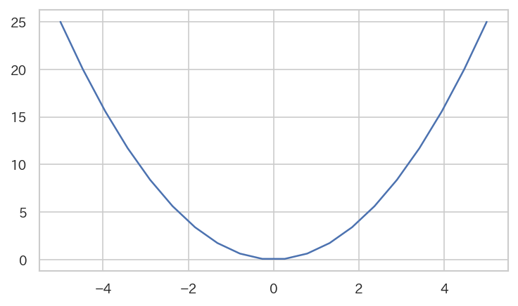
一番,シンプルな図は,以下のコードで作成出来る.
xx = np.linspace(-5,5,20)
yy = xx*xx

with BasicPlot() as p:
    p.ax.plot(xx,yy)
このコードで何が行われているかというと,with statement のBasicPlot()の部分で関数の初期化が行われる.context managerは処理に入るときと,出るときが,__enter__と__exit__ によって定義される.__enter__ で自分のclassを返すことで,pには BasicPlot() のインスタンスが代入される.そこで,インスタンスのアトリビュートに格納されているaxにアクセスして値を組み込んで描写させる.__exit__部分で図の表示まで行っているので,これだけで図を表示することが出来る.
メリットが出てくるのは,図を装飾していきたいときだ.冒頭の図と同じ図は以下のコードで生成することが出来る.
xx = np.linspace(-5,5,20)
yy = xx*xx

with BasicPlot(xlabel="xlabel",ylabel="ylabel",title="title",
               xlim=[-2,4],ylim=[0,20], figsize=(3,3),dpi=200,save_path="./test.png") as p:
    p.ax.plot(xx,yy)
わずか,3行で描写が可能になる.context managerを用いることで,keyword argumentsとして,図の設定を調整することが可能になるため,pythonの関数のような感覚で図の作成が出来る.
この方法での図の作成の良い点としては,同じ図の設定で,ax.plotの箇所の値だけ変えていきたい場合,短いコードで多くの図が作成出来る点だ.
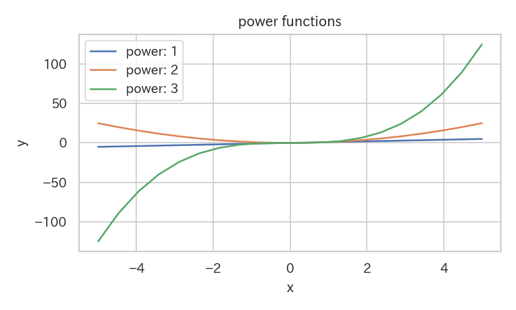
例えば,次のコードで指数部分を変えた関数を図示することが可能だ.
xx = np.linspace(-5,5,20)
y1 = xx**1
y2 = xx**2
y3 = xx**3
with BasicPlot(xlabel="x",ylabel="y",title="power functions",save_path="./power_func.png") as p:
    p.ax.plot(xx,y1,label="power: 1")
    p.ax.plot(xx,y2,label="power: 2")
    p.ax.plot(xx,y3,label="power: 3")
    plt.legend()
context mangerはclassで定義されているため,context 内部でmethod functionを用いて,図の描写を行うことは,もちろん可能である.以下の図は一個前のコードと全く同じ図を生成する.クラスを継承することによってメソッドを増やしている.
class PowerPlot(BasicPlot):
    def power_plot(self,xx,powers):
        for power in powers:
            y = np.power(xx,power)
            self.ax.plot(xx,y,label=f"power: {power}")
        plt.legend()

xx = np.linspace(-5,5,20)
with PowerPlot(xlabel="x",ylabel="y",title="power functions",save_path="./power_func.png") as p:
    p.power_plot(xx,[1,2,3])
Variadic Arguments (**kargs) を用いてラップする
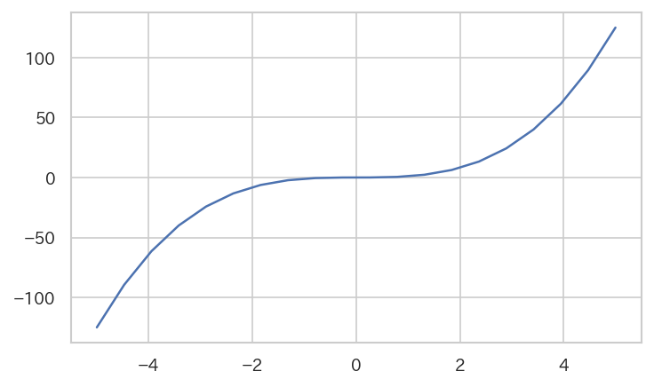
クラスの拡張ではなく,ある関数の中に今回のBasicPlotによる描写を組み込みたいとする.このときには,variadic argumentsを用いることによって引数を渡せば図の装飾を用意に変更することが可能となる.
シンプルな図の作成は,このコード.
def wrap_plot(power,**kargs):
    xx = np.linspace(-5,5,20)
    yy = np.power(xx,power)
    with BasicPlot(**kargs) as p:
        p.ax.plot(xx,yy)
wrap_plot(3)
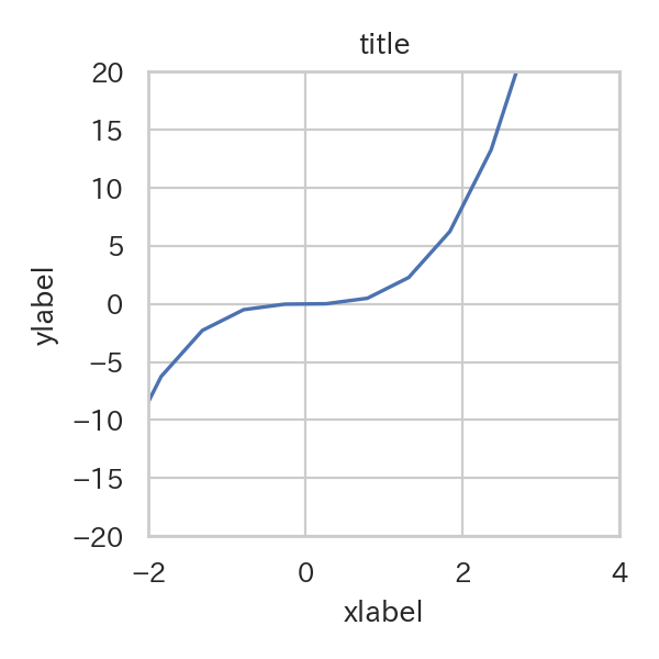
図を装飾するためには,以下のコード.辞書として引数を用意して,辞書を開いて関数に渡す.
dic_ = dict(xlabel="xlabel",ylabel="ylabel",title="title",
            xlim=[-2,4],ylim=[-20,20], figsize=(3,3),dpi=200,save_path="./kargs.png")
wrap_plot(3,**dic_)
x軸を日付にする
さて,次は,BasicPlotを更に拡張して,x軸が日付になる図を作成したい.この際に,BasicPlotで用意したoption methodを用いる.
import matplotlib.dates as mdates
class DatePlot(BasicPlot):
def __init__(self,rotation=90,x_fontsize=10,**kargs):
super().__init__(**kargs)
self.rotation = rotation
self.x_fontsize = x_fontsize
def option(self):
self.ax.xaxis.set_major_locator(mdates.DayLocator(bymonthday=None, interval=1, tz=None))
self.ax.xaxis.set_major_formatter(mdates.DateFormatter("%Y-%m-%d"))
plt.xticks(rotation=self.rotation,fontsize=self.x_fontsize)
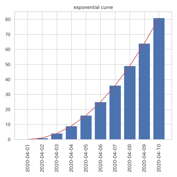
xx = [np.datetime64("2020-04-01")+np.timedelta64(i,"D") for i in range(10)]
yy = [i*i for i in range(10)]
with DatePlot(title="exponential curve",figsize=(5,5),save_path="./date.png") as p:
p.ax.plot(xx,yy,color="r")
p.ax.bar(xx,yy)
更に自分が頻繁に変える部分に関しては追加でclassを変更したり,拡張したり,関数の中に組み込んだりと工夫の余地がいっぱい広がる!
複数のグラフの描写
今までは,一つの図の場合を取り扱ったが,複数の場合に用いることが出来るclassをここで定義する.
class MultiPlot():
    def __init__(self, figsize=(8,6), dpi=150,grid=(2,2) ,suptitle="",
            save_path=None,show=True, tight=True):
        self.fig = plt.figure(figsize=figsize,dpi=dpi)
        self.grid = grid
        self.save_path = save_path
        self.show = show
        self.tight = tight

        plt.suptitle(suptitle)

    def set_ax(self,index,xlim=None, ylim=None, xlabel="", ylabel="",title=""):
        ax = self.fig.add_subplot(*self.grid,index)
        ax.set_xlabel(xlabel)
        ax.set_ylabel(ylabel)
        ax.set_xlim(xlim) if xlim else None
        ax.set_ylim(ylim) if ylim else None
        ax.set_title(title)
        return(ax)

    def __enter__(self):
        return(self)

    def __exit__(self,exc_type, exc_value, exc_traceback):
        self.option()
        plt.tight_layout() if self.tight else None
        plt.savefig(self.save_path) if self.save_path else None
        plt.show() if self.show else None

    def option(self):
        """This method is for additional graphic setting.
        See DatePlot for example."""
        pass
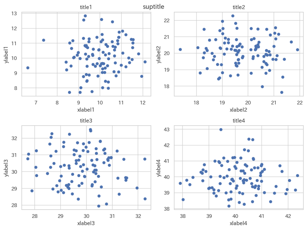
このクラスの使い方の例は例えば,以下のようにすれば良い.
with MultiPlot(suptitle="suptitle") as p:
    for i in range(1,5):
        ax = p.set_ax(i,xlabel=f"xlabel{i}",ylabel=f"ylabel{i}",title=f"title{i}")
        x = np.random.normal(i*10,1,size=100)
        y = np.random.normal(i*10,1,size=100)
        ax.scatter(x,y)
———-雑感(`・ω・´)———-
context managerを用いると図が非常に簡単に作れる!
元々,snippetを登録して作業していたが,次からは,moduleにこのclassを定義しといて,importして用いる形にしていこうと思う.
jupyter notebookのsnippetに関しては,自動で作成がおすすめ.
自動でjupyter notebookのsnippetを作成する!

コメント