
matplotlibを使った様々な図の紹介.
データ解析の際に良い図を作成するためには色々な設定が必要.
だけど, 自分が作りたい図を作るには結構なググる手間が必要.
そこで, 出来るだけバリエーションに富んだ図のギャラリーを先に用意してしまおうという次第. (備忘録の側面が強いです. )
ここでの紹介する図の条件
・seabornはグラフの体裁を整えるためのみ使う. 極力使用は避ける
・pandasの描写機能は使わない
どの画像作成時にも冒頭に以下の設定を入れている.
import pandas as pd
import numpy as np
import matplotlib.pyplot as plt
%matplotlib inline
import seaborn as sns
sns.set(context="paper" , style ="whitegrid",rc={"figure.facecolor":"white"})
紹介する図はjupyter notebook上で出来を確認している. なので実行する環境もjupyter notebook上をお勧めする.
画像で保存する際に端が見切れてしまうなどがあれば, plt.tight_layout() の一行を入れると良い感じに調整が入る.
ギャラリー
*右にある〜画像n〜 の部分を押すとコードが載っている場所まで飛びます.
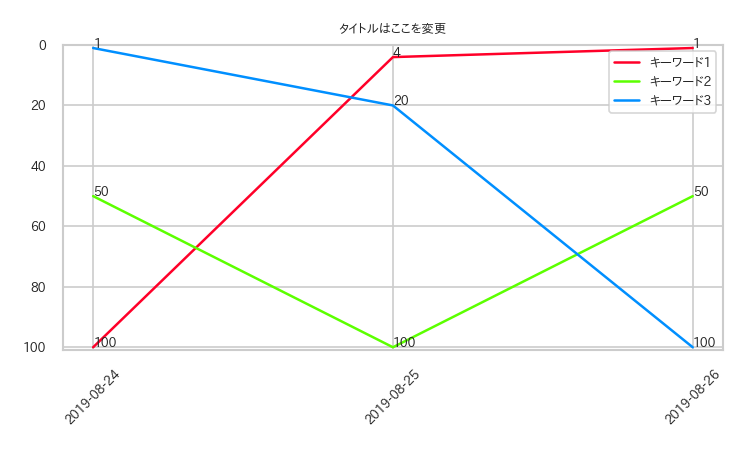
〜画像1〜
・x軸を日付
・y軸を反対向き
・colormapをgist_rainbow
・図に日本語を入れる
・点の近くに文字をつける
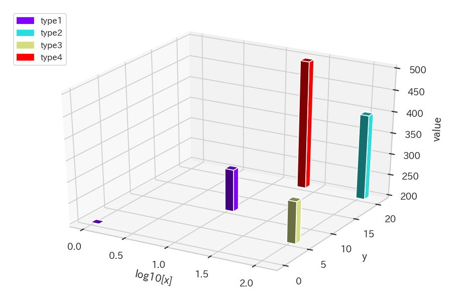
〜画像2〜
・3dのbar plot
・z軸は最小の値を基準
・凡例を一から自作
・凡例の位置調整
・x軸は対数

〜画像3〜
・複数の図の配置
・複数の図に対するタイトルの入れ方
・論文に使えるmatplotlibの設定
・タイトルへのindexの振り方( (A), (B)…など)
・信頼区間の作成
・図の軸を合わせる
・複数図の調節の仕方(plt.subplots_adjustによる方法)
・水平線, 垂直線の挿入
・凡例の位置の調節
・colormapはtab10
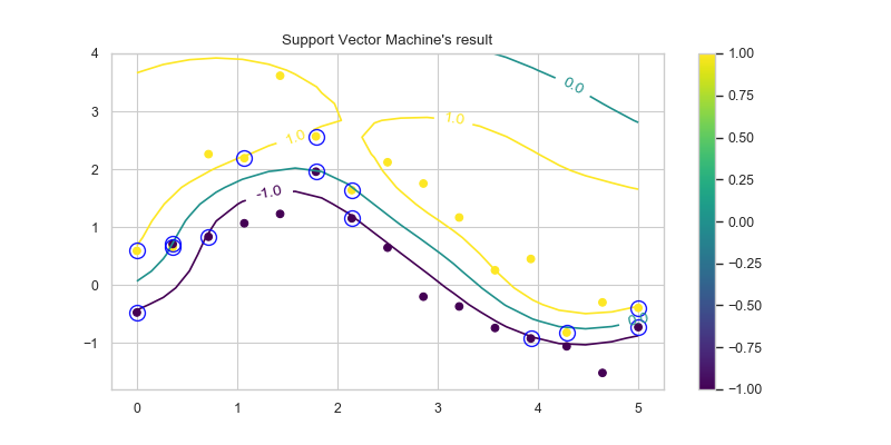
〜画像4〜
・scatter plotでの点ごとの色の設定
・カラーバーの表示
・中抜きの点の作成
・等高線図の作成
・等高線に値を表示させる
画像と画像作成用のコード
画像1
・x軸を日付
・y軸を反対向き
・colormapをgist_rainbow
・図に日本語を入れる
・点の近くに文字をつける
from datetime import datetime
from datetime import timedelta
import matplotlib.dates as mdates

####### preparing data for plot #######
url = "url, ex:https://xxxxx"
title = "タイトルはここを変更"
keywords = ["キーワード1","キーワード2","キーワード3"]

# convert date to the start of the date, i.e., AM0:00.
s = datetime.strftime(datetime.today(),"%Y%m%d")
today = datetime.strptime(s,"%Y%m%d")
delta = timedelta(days=1)
days = [today, today +delta,today + delta*2]
ranks = [{"date":days,"rank":[100,4,1]},
        {"date":days,"rank":[50,100,50]},
        {"date":days,"rank":[1,20,100]}
       ]
rankMax = 100

####### plot part #######
fig = plt.figure(figsize=(5,3),dpi=150)
# 図に日本語を入れる
plt.rcParams['font.family'] = 'IPAPGothic'
# colormapの設定
cmap = plt.get_cmap("gist_rainbow")
n = len(ranks)
c = [cmap(i/n) for i in range(n) ]
ax = fig.add_subplot(111)

for keyword, rank,cc in zip(keywords,ranks,c):
    ax.plot(rank["date"],rank["rank"] ,label=keyword,c=cc)
    # 点の近くに文字をつける
    for i in range(len(rank["rank"])):
        ax.annotate(str(rank["rank"][i]),(rank["date"][i],rank["rank"][i]),fontsize=6)

ax.set_ylim(0,rankMax + 1)
# y軸を反対向きに
ax.invert_yaxis()

# x軸を日付に
ax.xaxis.set_major_locator(mdates.DayLocator(bymonthday=None, interval=1, tz=None))
ax.xaxis.set_major_formatter(mdates.DateFormatter("%Y-%m-%d"))
labels = ax.get_xticklabels()
plt.setp(labels, rotation=45, fontsize=6)


plt.rcParams["ytick.labelsize"] = 6.0
ax.set_title(title,fontsize = 6)
ax.legend(fontsize = 6)
plt.tight_layout()
plt.show()
参考文献
・matplotlib.datesで時系列データのグラフの軸目盛の設定をする , https://bunseki-train.com/setting_ticks_by_matplotlib_dates/
・color example code: colormaps_reference.py, https://matplotlib.org/examples/color/colormaps_reference.html
画像2
・3dのbar plot
・z軸は最小の値を基準
・凡例を一から自作
・凡例の位置調整
・x軸は対数
・colormapはrainbow
import matplotlib.patches as mpatches
from mpl_toolkits.mplot3d import Axes3D

###### preparing data for plot ######
data = {'value': [200, 300, 400, 300, 500],
 'x': [1, 10, 100, 100, 20],
 'y': [0 ,10, 20, 5, 20],
 'type': [0, 0, 1, 2, 3]}

###### plot part ######
fig = plt.figure(figsize=(6,4),dpi=150)
# 3d plotの設定
ax1 = fig.add_subplot(111, projection='3d')

# preparing data for 3d plot
n = len(data["x"])
zpos = [np.min(data["value"])  for i in range(n)]
dx = np.full(n,0.1)
dy = np.full(n,1)

# colormapはrainbow
cm = plt.get_cmap('rainbow')
col = np.array(data["type"])/3

# 3dのbar plot
# z軸は最小の値を基準
# x軸は対数
ax1.bar3d(np.log10(data["x"]), np.array(data["y"]),zpos,
          dx,dy, data["value"] - np.min(data["value"]) ,color = cm(col))

ax1.set_xlabel("log10[x]")
ax1.set_ylabel("y")
ax1.set_zlabel("value")
# 凡例を一から自作
col_t  = np.array([0,1,2,3])/3
col_l = ["type1","type2","type3","type4"]
patch = []
for i in range(4):
    patch.append(mpatches.Patch(color=cm(col_t[i]), label=col_l[i] ))
# 凡例の位置調整
plt.legend(handles=patch,bbox_to_anchor=(0, 1), loc='upper left', borderaxespad=0, fontsize=8)
plt.tight_layout()
plt.show()
画像3
・複数の図の配置
・複数の図に対するタイトルの入れ方
・論文に使えるmatplotlibの設定
・タイトルへのindexの振り方( (A), (B)…など)
・信頼区間の作成
・図の軸を合わせる
・複数図の調節の仕方(plt.subplots_adjustによる方法)
・水平線, 垂直線の挿入
・凡例の位置の調節
・colormapはtab10
*個別の図に関する注釈は, 右上の図の場所にのみ入れてある.
####### data preparation for plot ######
d = {"t":[2004,2005,2006,2007,2008,2009,2010],
     "mean":[0.5 ,1.0 ,1.5 ,1.0 ,0.5 ,1 ,1.5],
     "l":[0.3 ,0.5 ,1 ,0.3 ,0.1 ,0.8 ,1.2],
     "h":[0.9 ,1.3 ,2 ,1.2 ,0.9 ,2.0 ,1.8]}
d1 = {"t":[2004,2005,2006,2007,2008,2009,2010],
     "mean":[0.5 ,1.0 ,1.5 ,1.0 ,0.5 ,1 ,1.5],
     "l":[0.3 ,0.5 ,1 ,0.3 ,0.1 ,0.8 ,1.2],
     "h":[0.9 ,1.3 ,2 ,1.2 ,0.9 ,2.0 ,1.8]}
d1["mean"] = [i + 0.5 for i in d["mean"]]
d1["l"] = [i + 0.4 for i in d["l"]]
d1["h"] = [i + 0.6 for i in d["h"]]

# 論文に使えるmatplotlibの設定
plt.rcParams['font.size'] = 8
plt.rcParams['font.family']= 'sans-serif'
plt.rcParams['font.sans-serif'] = ['Arial']
plt.rcParams['xtick.direction'] = 'in'
plt.rcParams['xtick.labelsize'] = 7
plt.rcParams['ytick.direction'] = 'in'
plt.rcParams['ytick.labelsize'] = 7
plt.rcParams['xtick.major.width'] = 1.2
plt.rcParams['ytick.major.width'] = 1.2
plt.rcParams['axes.linewidth'] = 1.2
plt.rcParams['axes.grid']=True
plt.rcParams['grid.linestyle']='--'
plt.rcParams['grid.linewidth'] = 0.3
plt.rcParams["legend.markerscale"] = 2
plt.rcParams["legend.fancybox"] = False
plt.rcParams["legend.framealpha"] = 1
plt.rcParams["legend.edgecolor"] = 'black'

# colormapはtab10
cm = plt.get_cmap("tab10")
col = [0,1]
xlim = [2002,2011]


fig = plt.figure(figsize=(8,10),dpi=300)

# 複数の図の配置
#### figure top left ####
ax = fig.add_subplot(3,2,1)
# dataのセット
d_ = d
ax.plot(d_["t"],d_["mean"],label = "kind1")
# 信頼区間の作成
ax.fill_between(d_["t"],d_["l"],d_["h"],alpha = 0.1)
# 2セット目のデータ
d_ = d1
ax.plot(d_["t"],d_["mean"],label = "kind2")
# 信頼区間の作成
ax.fill_between(d_["t"],d_["l"],d_["h"],alpha = 0.1)

# 図の軸を合わせる
ax.set_ylim([0,5])
ax.set_xlim(xlim[0],xlim[1])
ax.set_title("Country(A)",fontsize=10)
# タイトルへのindexの振り方( (A), (B)...など)
ax.set_title("(A)",loc ="left")

ax.set_ylabel("specific value",fontsize = 10)
# 点線の水平線の挿入
ax.axhline(y = 1,color = "black",alpha = 0.5,linestyle = ":")
# 垂直線の挿入
ax.axvline(x = 2009,color = "red",alpha = 0.5,linestyle = "dashdot")
# 凡例の位置の調節
ax.legend(bbox_to_anchor=(0.6, 0.98), loc='upper left', borderaxespad=0, fontsize=8,frameon = False)


###### middle left ######
ax = fig.add_subplot(3,2,3)
d_ = d
ax.plot(d_["t"],d_["mean"],label="kind3")
ax.fill_between(d_["t"],d_["l"],d_["h"],alpha = 0.1)
d_ = d1
ax.plot(d_["t"],d_["mean"],label = "kind4")
ax.fill_between(d_["t"],d_["l"],d_["h"],alpha = 0.1)

ax.set_ylim([0,5])
ax.set_xlim(xlim[0],xlim[1])
ax.set_title("Country(B)",fontsize=10)
ax.set_title("(B)",loc ="left")
ax.set_ylabel("specific value",fontsize = 10)
ax.axhline(y = 1,color = "black",alpha = 0.5,linestyle = ":")
ax.legend(bbox_to_anchor=(0.6, 0.98), loc='upper left', borderaxespad=0, fontsize=8,frameon = False)


###### bottom left #####
ax = fig.add_subplot(3,2,5)
d_ = d
ax.plot(d_["t"],d_["mean"])
ax.fill_between(d_["t"],d_["l"],d_["h"],alpha = 0.1)
ax.set_ylim([0,5])
ax.set_xlim(xlim[0],xlim[1])

ax.set_title("Country(C)",fontsize=10)
ax.set_title("(C)",loc ="left")
ax.set_ylabel("specific value",fontsize = 10)
ax.set_xlabel("Year",fontsize = 10)
ax.axhline(y = 1,color = "black",alpha = 0.5,linestyle = ":")

###### top right #####
ax = fig.add_subplot(3,2,2)
d_ = d1
ax.plot(d_["t"],d_["mean"],label = "kind5")
ax.fill_between(d_["t"],d_["l"],d_["h"],alpha = 0.1)
d_ = d
ax.plot(d_["t"],d_["mean"],label = "kind6")
ax.fill_between(d_["t"],d_["l"],d_["h"],alpha = 0.1)

ax.set_ylim([0,5])
ax.set_xlim(xlim[0],xlim[1])
ax.set_title("Country(D)",fontsize=10)
ax.set_title("(D)",loc ="left")
ax.axhline(y = 1,color = "black",alpha = 0.5,linestyle = ":")
ax.legend(bbox_to_anchor=(0.53, 0.98), loc='upper left', borderaxespad=0, fontsize=8,frameon = False)

###### middle right #####
ax = fig.add_subplot(3,2,4)
d_ = d1
ax.plot(d_["t"],d_["mean"])
ax.fill_between(d_["t"],d_["l"],d_["h"],alpha = 0.1)
ax.set_ylim([0,5])
ax.set_xlim(xlim[0],xlim[1])

ax.set_title("Country(E)",fontsize=10)
ax.set_title("(E)",loc ="left")
ax.axhline(y = 1,color = "black",alpha = 0.5,linestyle = ":")

###### bottom right #####
ax = fig.add_subplot(3,2,6)
d_ = d
ax.plot(d_["t"],d_["mean"])
ax.fill_between(d_["t"],d_["l"],d_["h"],alpha = 0.1)
ax.set_ylim([0,5])
ax.set_xlim(xlim[0],xlim[1])

ax.set_title("Country(F)",fontsize=10)
ax.set_title("(F)",loc ="left")
ax.set_xlabel("Year",fontsize = 10)
ax.axhline(y = 1,color = "black",alpha = 0.5,linestyle = ":")

# 複数図の調節の仕方
plt.subplots_adjust(hspace = 0.3)
# 複数の図に対するタイトルの入れ方
plt.suptitle("Title for All",fontsize=14)
plt.show()
参考文献
・[Matplotlib] 線の種類、色と太さの設定, https://python.atelierkobato.com/linestyle/
画像4
・scatter plotでの点ごとの色の設定
・カラーバーの表示
・中抜きの点の作成
・等高線図の作成
・等高線に値を表示させる
データは図のコードの後に載せています.
d : オリジナルデータ,
t : 二値データを表すラベル
M_ind : 分類に用いたベクトル(特定の点の選択)
xx, yy, zz : 等高図作成のためのデータ
plt.figure(figsize=(8,4),dpi=100)
# scatter plotでの点ごとの色の設定
plt.scatter(d.T[0],d.T[1],c = t, cmap="viridis")
# カラーばーの表示
plt.colorbar()
# 中抜きの点の作成
plt.plot(d.T[0][M_ind],d.T[1][M_ind],alpha = 0.9,marker="o",color = "none",
            markeredgewidth=1,markersize=10,markeredgecolor="blue")
# 等高線図の作成
cont = plt.contour(xx,yy,zz,levels=[-1,0,1],alpha = 1,cmap="viridis")
# 等高線に値を表示させる
cont.clabel(fmt="%1.1f")

plt.title("Support Vector Machine's result")
plt.savefig("figures/picture4.png")
###### data preparation ######
d = [[ 0.         , 0.58792136],
 [ 0.35714286 , 0.65059507],
 [ 0.71428571 , 2.2589972 ],
 [ 1.07142857 , 2.18893163],
 [ 1.42857143 , 3.61438134],
 [ 1.78571429 , 2.56540189],
 [ 2.14285714 , 1.63760114],
 [ 2.5        , 2.11924754],
 [ 2.85714286 , 1.75131123],
 [ 3.21428571 , 1.16447881],
 [ 3.57142857 , 0.25268311],
 [ 3.92857143 , 0.44806573],
 [ 4.28571429 ,-0.82397943],
 [ 4.64285714 ,-0.30254881],
 [ 5.         ,-0.39698456],
 [ 0.         ,-0.47722782],
 [ 0.35714286 , 0.70627337],
 [ 0.71428571 , 0.83138323],
 [ 1.07142857 , 1.06416043],
 [ 1.42857143 , 1.2261952 ],
 [ 1.78571429 , 1.95625809],
 [ 2.14285714 , 1.15018027],
 [ 2.5        , 0.64314441],
 [ 2.85714286 ,-0.20412688],
 [ 3.21428571 ,-0.37272828],
 [ 3.57142857 ,-0.74467096],
 [ 3.92857143 ,-0.92585504],
 [ 4.28571429 ,-1.06192697],
 [ 4.64285714 ,-1.52131693],
 [ 5.         ,-0.73024455]]
d = np.array(d)
zz = [[-1.61807684, -1.633405  , -1.58946098, -1.51001585, -1.43002277,
        -1.38879342, -1.42112656, -1.54741758, -1.76453094, -2.04067112,
        -2.31852779, -2.52970711, -2.61878679, -2.56867967, -2.41451957,
        -2.2355021 , -2.12403896, -2.14456411, -2.30214174, -2.53756996],
       [-1.74146737, -1.79695082, -1.79249889, -1.74788025, -1.69488607,
        -1.67105559, -1.71059436, -1.83346193, -2.03480379, -2.27876817,
        -2.50192621, -2.62988208, -2.60507508, -2.41599685, -2.11289748,
        -1.79768684, -1.58727147, -1.56462716, -1.74104035, -2.04912408],
       [-1.66018946, -1.78542633, -1.86239281, -1.8990248 , -1.91490826,
        -1.93758259, -1.99496556, -2.10445949, -2.26119212, -2.4302707 ,
        -2.54928029, -2.54531098, -2.36449734, -2.00344107, -1.52621218,
        -1.05340322, -0.72212673, -0.63214792, -0.80341916, -1.16653549],
       [-1.34649219, -1.57473552, -1.77994591, -1.94925579, -2.07983109,
        -2.18018843, -2.26621484, -2.3515418 , -2.43479243, -2.48941465,
        -2.46345894, -2.29453562, -1.93842415, -1.40068028, -0.75450003,
        -0.13064367,  0.32238751,  0.49320681,  0.35216929, -0.03634755],
       [-0.8388561 , -1.19842971, -1.57102796, -1.91499279, -2.19608646,
        -2.39613313, -2.51470271, -2.56202016, -2.54534613, -2.45528969,
        -2.26069213, -1.91866066, -1.39938238, -0.71594386,  0.05711217,
         0.79089826,  1.33789258,  1.58339976,  1.48934232,  1.10901945],
       [-0.23422925, -0.73752393, -1.2944945 , -1.83016367, -2.27369078,
        -2.57589708, -2.71824924, -2.70946231, -2.5711947 , -2.3197966 ,
        -1.95415925, -1.45809045, -0.81876978, -0.05323704,  0.77219661,
         1.54399333,  2.12939478,  2.42054116,  2.37456356,  2.03014378],
       [ 0.34955615, -0.28429248, -1.00975681, -1.71945087, -2.30628046,
        -2.690153  , -2.83516515, -2.75093922, -2.47812308, -2.06501954,
        -1.54679979, -0.93808736, -0.24316857,  0.52178565,  1.30805677,
         2.02965533,  2.58103087,  2.87106255,  2.8572705 ,  2.56324935],
       [ 0.82326765,  0.10137827, -0.74210004, -1.57441371, -2.25840358,
        -2.68723311, -2.80984271, -2.63800133, -2.23268185, -1.6759435 ,
        -1.04093328, -0.37353066,  0.30672791,  0.98909875,  1.64935316,
         2.23735712,  2.68328729,  2.92024093,  2.911391  ,  2.66734989],
       [ 1.15988604,  0.41686238, -0.46857891, -1.35050728, -2.07246624,
        -2.5077436 , -2.59234693, -2.33869135, -1.82459497, -1.16196982,
        -0.4584018 ,  0.21205943,  0.81745678,  1.35517221,  1.82806345,
         2.22446425,  2.51319731,  2.6550635 ,  2.62279042,  2.41754537],
       [ 1.39282079,  0.70671127, -0.13601975, -0.99116704, -1.69605101,
        -2.11199923, -2.16337591, -1.85856971, -1.28378496, -0.57118999,
         0.14568693,  0.77060528,  1.26204929,  1.62535314,  1.88795123,
         2.07307325,  2.18517939,  2.21178488,  2.13684322,  1.95584551],
       [ 1.581239  ,  1.02364287,  0.29817896, -0.46711621, -1.11624806,
        -1.50638815, -1.5508531 , -1.24740903, -0.67887509,  0.01602632,
         0.69003468,  1.23276043,  1.59563079,  1.78898182,  1.85781351,
         1.85148604,  1.80220604,  1.71939772,  1.59761382,  1.42983414],
       [ 1.76556641,  1.38550428,  0.8274738 ,  0.1923268 , -0.38135814,
        -0.7538615 , -0.82863041, -0.58686566, -0.09605199,  0.51344433,
         1.09449619,  1.53175364,  1.77197833,  1.82602192,  1.74686699,
         1.59826731,  1.42946611,  1.26464774,  1.10662399,  0.94806286],
       [ 1.94080819,  1.75515606,  1.38407153,  0.89558764,  0.40357227,
         0.03796394, -0.0979797 ,  0.03368163,  0.38946054,  0.8600706 ,
         1.31153431,  1.63281621,  1.7688149 ,  1.72671264,  1.55794436,
         1.32876052,  1.09438714,  0.88604984,  0.71165525,  0.56479073],
       [ 2.06164948,  2.05455534,  1.86101388,  1.51648152,  1.10677117,
         0.74619243,  0.53908514,  0.54027336,  0.73326216,  1.03760922,
         1.34228262,  1.54867875,  1.60327635,  1.5072599 ,  1.30340369,
         1.05093933,  0.80188101,  0.58778174,  0.41851537,  0.28903883],
       [ 2.0722426 ,  2.20271181,  2.15571175,  1.93928907,  1.61167629,
         1.26718084,  1.00408113,  0.88753068,  0.92501167,  1.06652477,
         1.22898931,  1.33195342,  1.3271685 ,  1.20992226,  1.01090156,
         0.77670452,  0.55017672,  0.35851367,  0.21108914,  0.10415897],
       [ 1.93993988,  2.15433974,  2.21111821,  2.09903769,  1.85234695,
         1.54325549,  1.25723371,  1.06113515,  0.97908246,  0.9876324 ,
         1.03157915,  1.05110828,  1.0063236 ,  0.88860999,  0.71669955,
         0.52301575,  0.33882466,  0.18463827,  0.06783007, -0.01436948],
       [ 1.67349295,  1.91876657,  2.03459677,  1.99924948,  1.82856109,
         1.57324907,  1.30151798,  1.07398215,  0.92255241,  0.84307602,
         0.80407819,  0.76556915,  0.69763975,  0.59047235,  0.45335235,
         0.30610336,  0.1689142 ,  0.05535118, -0.02974325, -0.08851868],
       [ 1.3187187 ,  1.55262033,  1.68874014,  1.70236527,  1.5971056 ,
         1.40518464,  1.17632743,  0.9597199 ,  0.78735099,  0.66628421,
         0.58241797,  0.51224709,  0.43571104,  0.34405119,  0.2404597 ,
         0.13535798,  0.04011504, -0.03753512, -0.09506797, -0.13426198],
       [ 0.93827291,  1.13451846,  1.26301686,  1.30121769,  1.24607604,
         1.1157483 ,  0.94323496,  0.76453062,  0.60670729,  0.4812304 ,
         0.38476022,  0.30569768,  0.23223481,  0.15788292,  0.0827245 ,
         0.01121154, -0.0512853 , -0.10115925, -0.13758226, -0.16207048],
       [ 0.58868075,  0.73688289,  0.84211078,  0.88655724,  0.86469106,
         0.78526747,  0.66814236,  0.53718283,  0.4125096 ,  0.30546977,
         0.21805142,  0.14603799,  0.08354813,  0.02652954, -0.02601861,
        -0.07282757, -0.11200243, -0.14239767, -0.16417232, -0.17859074]]

x = np.linspace(0,5,20)
y = np.linspace(-1.5,4,20)
xx,yy = np.meshgrid(x,y)
M_ind = [ 0,  1,  3,  5,  6, 12, 14, 15, 16, 17, 20, 21, 26, 29]

t = np.array([1 for i in range(15)] + [-1 for i in range(15)])

コメント
[…] 以前,matplotlibのギャラリーを少し書いたが,いちいちコードを載せるのが面倒だった.そこで,この記事では,画像だけを載せ,コードに関しては,githubへのリンクを直接紐付けるよう […]