
この記事では,plotlyを用いた図の作成について,基本的なものから,少し凝った図の作成方法を紹介する. どのようなことが出来るかは公式ドキュメントのExamples を参照のこと.
方針としては公式ドキュメントの各論を踏まえた上でよく使いそうな方法やメソッドをまとめた図を作成するようにした.
また,棒グラフなどはドキュメントでは既にまとめてあるデータが示されているが,ここではデータの加工から行った.1~3行でまとめる方法を紹介しているのでそこにも注目されたい.
画像をクリックすると該当箇所まで進めるようになっている.
また,以下のmoduleはimportされているものとする.
import plotly.express as px
import plotly.graph_objects as go
import pandas as pd
import numpy as np
なぜplotlyか
なぜ僕がplotlyをまとめたかというと,”10 Useful Python Data Visualization Libraries for Any Discipline” で紹介されていたlibrariesの中で,ドキュメントが分かりやすく,かつ,出来ることが多いように感じたからだ(特にparallelSetの図を描きたかった).
plotlyはjavaScriptで提供されている機能をpythonでwrapして提供することにより,visualizationの分野で秀でているjavaScriptの恩恵をpythonでも享受しようという野心がある.そのため,matplotlibには見られないinteractiveな図の探索が基本的な図に既に搭載されている.そのため,探索的なデータ解析で値を調べるために元データに戻る作業をしなくて済む.
それぞれのFigureをもっと細かく調整したい場合はplotlyの Python Figure Reference を調べると良い.
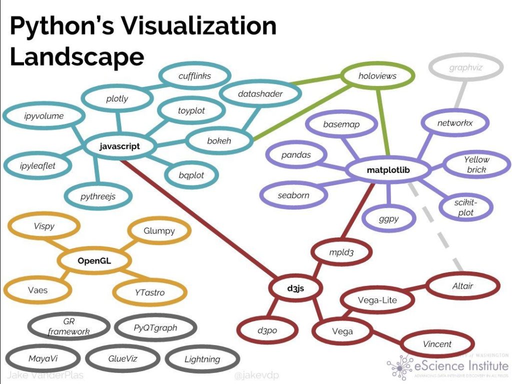
pythonのvisualization toolsの比較については,Python Data Visualization 2018: Why So Many Libraries? 参照のこと.以下にこのサイトより拝借した図を掲載する.
ギャラリー
Scatter Plots / 散布図
simple scatter 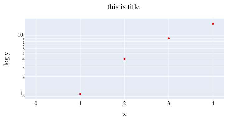
decorated scatter 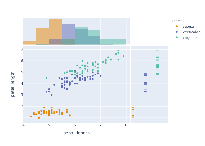
stratified scatter 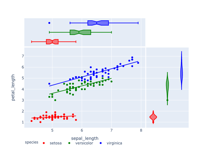
scatter with linear reg. 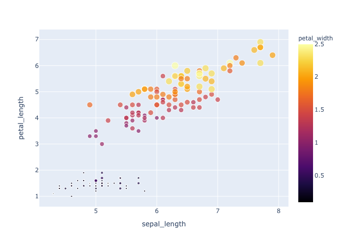
bubble chart
Line Charts / 折線グラフ
simple line chart 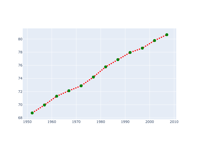
line chart with markers 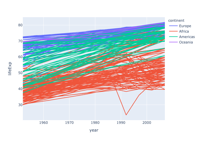
stratified line chart 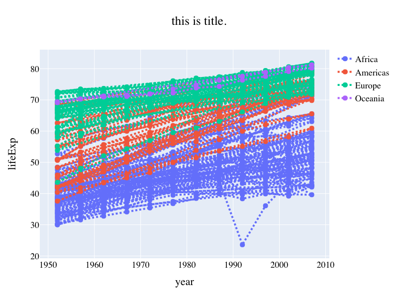
stratified with markers 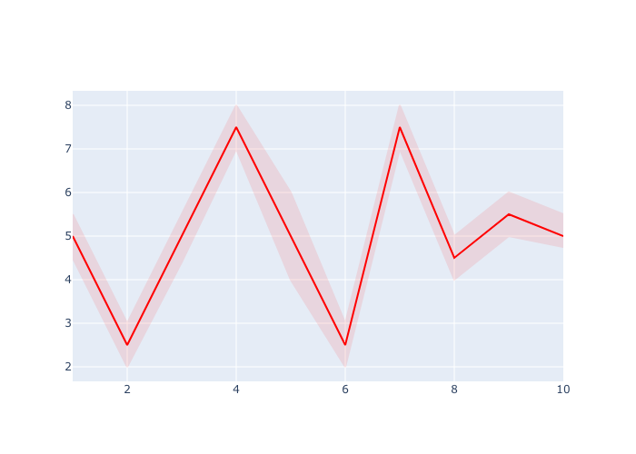
filled line chart
Bar Charts / 棒グラフ
simple bar chart 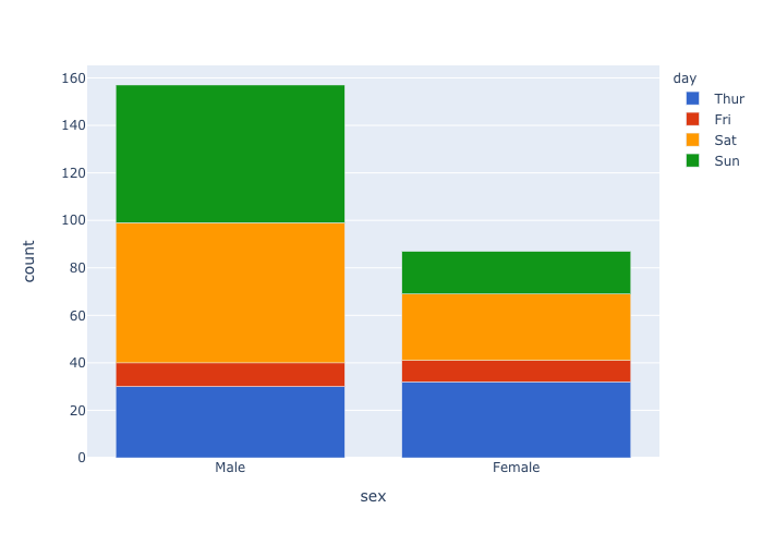
stacked bar chart 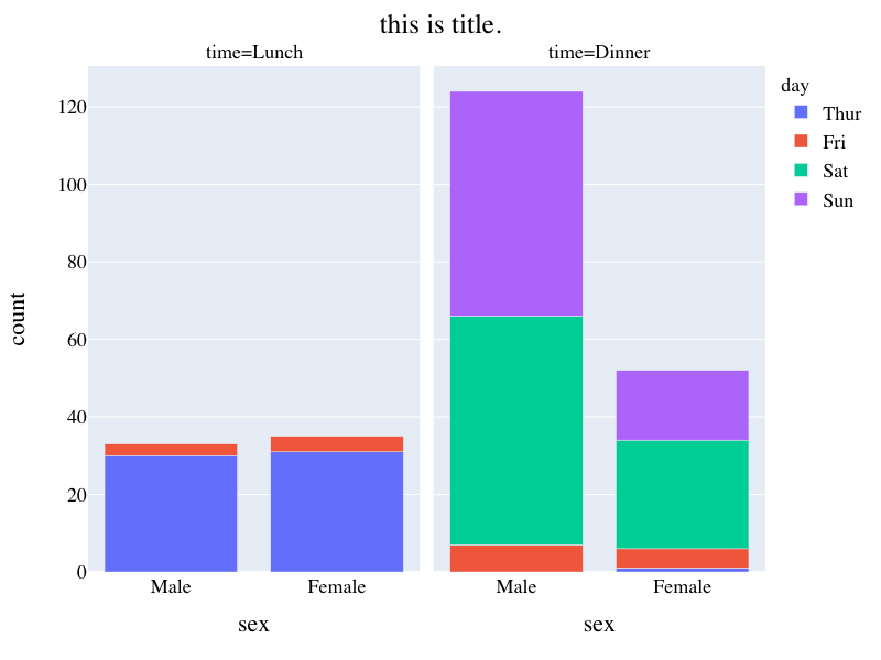
facet bar chart 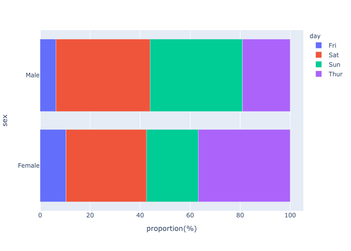
bar chart (%) 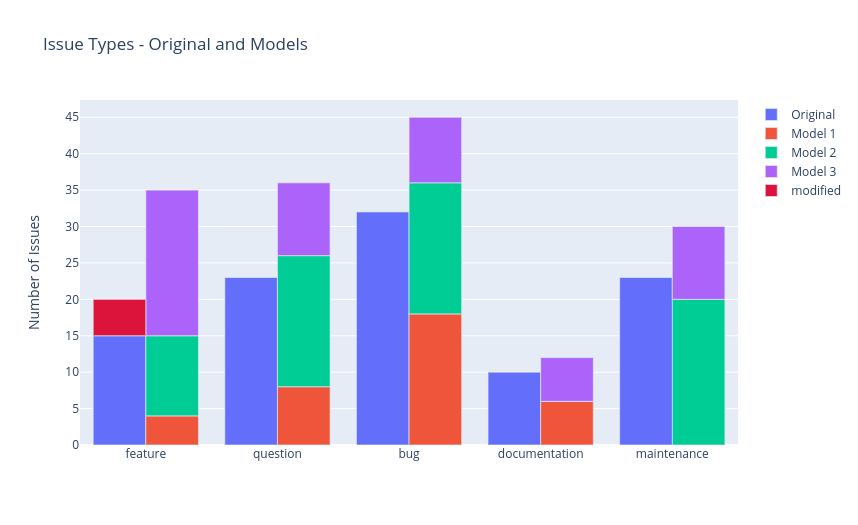
grouped stacked bar chart
3種類以上の変数の関係の可視化
sunburst 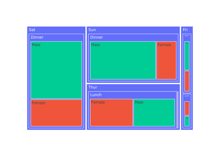
treemap 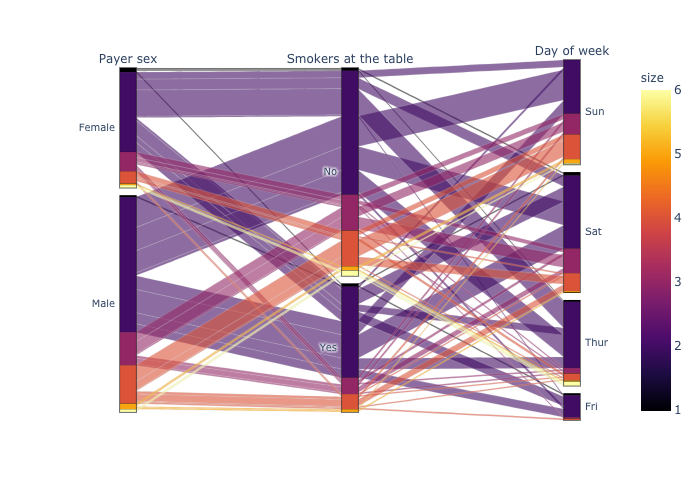
parallelSet1 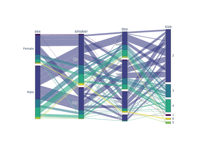
parallelSet2
図と図作成用のコード
Scatter Plots / 散布図
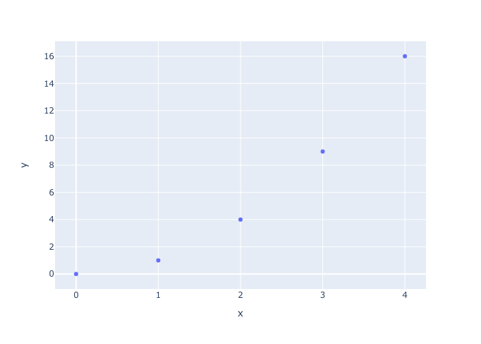
simple scatter plot

- simple scatter plot.
x =[0,1,2,3,4]
y = [0,1,4,9,16]
fig = px.scatter(x=x, y=y)
fig.show()
fig.write_image("pic/scatter1.png")
decorated scatter plot/散布図を修飾
- scatter plot
- 軸を対数,plotの色の変更,
- figure sizeの指定,タイトル・x軸・y軸の追加,
- タイトルの中央寄せ,
- フォントの大きさ,色調整.
x =[0,1,2,3,4]
y = [0,1,4,9,16]
fig = px.scatter(x=x, y=y,
                 log_y = True,
                 width = 800, height = 400,
                color_discrete_sequence=["red"])

fig.update_layout(title="this is title.",title_x=0.5,
                  xaxis_title = "x", yaxis_title="log y",
                  font=dict(family="Times",size=18,color="black"))
fig.show()
stratified scatter plot
- pandas dataframeを用いた図示
- 種類ごとに点を塗り分ける,
- colorscaleの指定,
- 周辺分布の指定(hist,rug).
df = px.data.iris()

fig = px.scatter(df,x="sepal_length", y="petal_length",
                 color="species",color_discrete_sequence=px.colors.qualitative.Vivid,
                 marginal_y ="rug", marginal_x="histogram")

fig.show()
scatter plot with a linear regression
- 離散変数での層別化の際にcolorをそれぞれ指定して塗り分ける,
- 周辺分布の指定(violin,box)
- 線形回帰の表示,
- legendを下に持ってくる.
df = px.data.iris()
fig = px.scatter(df,x="sepal_length", y="petal_length",
                 color="species", color_discrete_sequence=["red", "green", "blue"],
                 marginal_y="violin",marginal_x="box", trendline="ols"
            )
fig.update_layout(legend_orientation="h")
fig.show()
bubble chart
- bubble chart,
- 点を塗り分ける,
- colorscaleの指定(sequentialは名前指定可能),
- sizeの最大値を指定,
- カーソルを合わせた時に表示される名前を指定.
df = px.data.iris()
fig = px.scatter(df,x="sepal_length", y="petal_length",
                 color="petal_width",size = "petal_width",
                 color_continuous_scale="inferno",
                 size_max=10,hover_name="species")
fig.show()
Line Charts / 折れ線グラフ
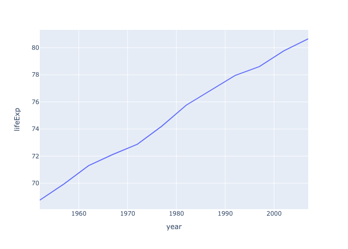
simple line chart
- simple line chart.
df = px.data.gapminder().query("country=='Canada'")
fig = px.line(df, x="year", y="lifeExp")
fig.show()
line chart with markers
- goを用いたline plot,
- lineにmarkerを付ける,
- lineとmarkerのpropertyを定める.
df = px.data.gapminder().query("country =='Canada'")
fig = go.Figure()
fig.add_trace(go.Scatter(x=df["year"], y=df["lifeExp"],
                         mode = "lines+markers",
                         line=dict(color="red",width=4,dash="dot"),
                         marker= dict(color="green",size=10)
            ))
fig.show()
stratified line chart
- 層別化して色を分ける.
df = px.data.gapminder().query("continent != 'Asia'") # remove Asia for visibility
fig = px.line(df, x="year", y="lifeExp", color="continent", hover_name="country")
fig.show()
stratified line chart with markers
- goを用いたline plot,
- lineにmarkerを付ける(goで処理する必要あり.),
- 国ごとに色を分ける,
- figure sizeの指定,タイトル・x軸・y軸の追加,
- タイトルの中央寄せ,フォントの大きさ,色調整.
df = px.data.gapminder().query("continent != 'Asia'") # remove Asia for visibility
fig = go.Figure()
cm = px.colors.qualitative.Plotly
x = "year"
y = "lifeExp"
for i,v  in enumerate(df.groupby("continent")):
    name,d = v
    fig.add_trace(go.Scatter(x=d[x], y=d[y],
                             mode = "lines+markers",
                             line=dict(color=cm[i],width=4,dash="dot"),
                             marker= dict(color=cm[i],size=10),
                             name = name
                            )
                 )
fig.update_layout(title="this is title.",title_x=0.5,
                  xaxis_title = x, yaxis_title=y,
                  font=dict(family="Times",size=18,color="black"),
                  width = 800, height = 600)
fig.show()
filled line chart
- filled lines,
- 透明度の指定,
- 追加したtraceのmodeを一括で変更,
- legendの非表示.
注 : plotly内でのfilled line chartsは一周して円を描いて範囲指定するようになっている.
x = [1, 2, 3, 4, 5, 6, 7, 8, 9, 10]
x_rev = x[::-1]
# Line 1
y1 = [5, 2.5, 5, 7.5, 5, 2.5, 7.5, 4.5, 5.5, 5]
y1_upper = [5.5, 3, 5.5, 8, 6, 3, 8, 5, 6, 5.5]
y1_lower = [4.5, 2, 4.4, 7, 4, 2, 7, 4, 5, 4.75]
y1_lower = y1_lower[::-1]


fig = go.Figure()
name = "filled_line"
fig.add_trace(go.Scatter(
    x=x+x_rev,
    y=y1_upper+y1_lower,
    fill='toself',
    fillcolor="red",
    line_color="red",
    opacity=0.1,
    name=name
))
fig.add_trace(go.Scatter(
    x=x, y=y1,
    line_color="red",
    name=name
))

fig.update_traces(mode='lines')
fig.update_layout(showlegend=False)

fig.show()
Bar Charts / 棒グラフ
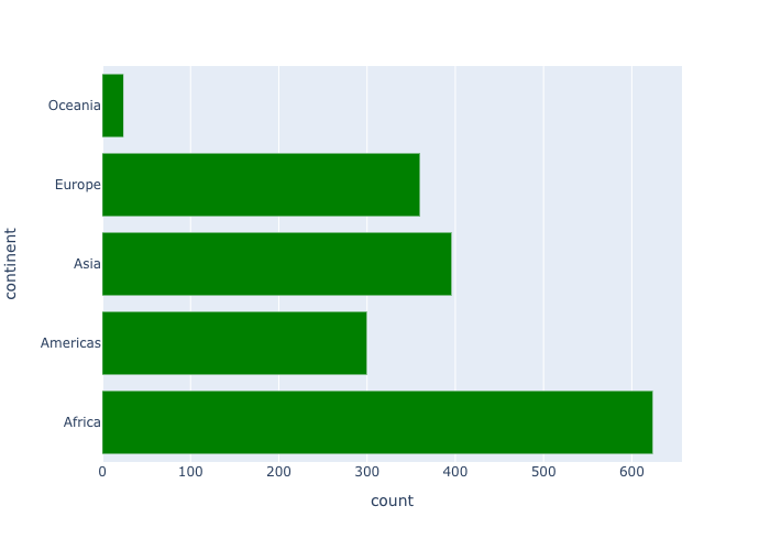
simple bar chart
- structured dataからbar chart用のデータ作成,
- simple bar chart,
- 色の変更,
- horizontalに向きを指定.
df = px.data.gapminder()
df["count"] = 1
dfM = df.groupby("continent",as_index=False)["count"].sum()
fig = px.bar(dfM,x="count",y="continent",color_discrete_sequence=["green"],orientation="h")
fig.show()
stacked bar chart
- structured dataからbar chart用のデータ作成,
- stacked bar chart,
- categoryのorderの指定,
- colorscaleの指定.
df = px.data.tips()
df["count"] = 1
dfM = df.groupby(["day","sex"],as_index=False)["count"].sum()

fig = px.bar(dfM, x="sex", y="count",color='day', barmode='relative',
            color_discrete_sequence=px.colors.qualitative.G10,
            category_orders={"sex":["Male","Female"],
                            "day":["Thur","Fri","Sat","Sun"]},
            )
fig.show()
facet bar chart
- structured dataからbar chart用のデータ作成,
- Facet stacked bar chart,
- categoryのorderの指定,
- hover時の表示されるデータの追加,
- figure sizeの指定,タイトルの追加
- タイトルの中央寄せ,フォントの大きさ,色調整.
df = px.data.tips()
df["count"] = 1
dfM = df.groupby(["time","day","sex"],as_index=False)["count","total_bill"].sum()

fig = px.bar(dfM, x="sex", y="count",color='day', barmode='relative',
             facet_col="time", hover_data=["total_bill"],
             category_orders={"sex":["Male","Female"],
                            "day":["Thur","Fri","Sat","Sun"],
                            "time":["Lunch","Dinner"]}
            )
fig.update_layout(title="this is title.",title_x=0.5,
                  font=dict(family="Times",size=18,color="black"),
                  width = 800, height = 600)
fig.show()
bar chart (%)
- structured dataからパーセントのデータ作成
- stacked bar chart(%),
- colorscaleの指定,
- horizontalに向きを指定,
- figure sizeの指定,タイトルの追加,
- タイトルの中央寄せ,フォントの大きさ,色調整.
df = px.data.tips()
df["count"] = 1
dfM = df.groupby(["day","sex"])["count"].sum()
dfM = dfM.groupby(level=1).apply(lambda x: 100*x/x.sum()).reset_index()
dfM = dfM.rename(columns={"count":"proportion(%)"})

fig = px.bar(dfM, x="proportion(%)",y="sex",color='day', barmode='relative',orientation="h" )
fig.show()
grouped stacked bar chart
・stacked bar chart をグループごとに設定.
・自分が望む位置に棒を設定可能.
data = {
    "original":[15, 23, 32, 10, 23],
    "model_1": [4,   8, 18,  6,  0],
    "model_2": [11, 18, 18,  0,  20],
    "model_3": [20, 10, 9,  6,  10],
    "labels": [
        "feature",
        "question",
        "bug",
        "documentation",
        "maintenance"
    ]
}

fig = go.Figure(
    data=[
        go.Bar(
            name="Original",
            x=data["labels"],
            y=data["original"],
            offsetgroup=0,
        ),
        go.Bar(
            name="Model 1",
            x=data["labels"],
            y=data["model_1"],
            offsetgroup=1,
        ),
        go.Bar(
            name="Model 2",
            x=data["labels"],
            y=data["model_2"],
            offsetgroup=1,
            base=data["model_1"],
        ),
        # NEW CODE
        go.Bar(
            name="Model 3",
            x=data["labels"],
            y=data["model_3"],
            offsetgroup=1,
            base=[val1+val2 for val1, val2 in zip(data["model_1"],data["model_2"])],
        ),
        # END NEW CODE
        go.Bar(
            name="modified",
            x=["feature"],
            y=[5],
            offsetgroup=0,
            base=[15],
            marker_color = ["crimson"],
        ),
    ],
    layout=go.Layout(
        title="Issue Types - Original and Models",
        yaxis_title="Number of Issues"
    )
)

fig.show()
3種類以上の変数の関係の可視化
うまく多変量のデータを可視化出来る方法としては,sunburst chart, treemap chart, parallelSetが代表的なのでここではその3つについて紹介する.
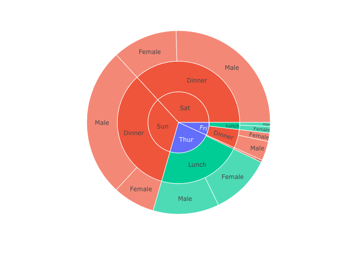
sunburst
- sunburst chart,
- 特定のカテゴリー(今回はLunchとDinner)で色分け.
df = px.data.tips()
fig = px.sunburst(df, path=['day', 'time', 'sex'], values='total_bill',color="time")
fig.show()
treemap
- treemap,
- 構造化データから必要なデータの作成,
- 特定のカテゴリーで色分け(今回は性別).
df = px.data.tips()
df["count"] = 1
dfM = df.groupby(by=['day', 'time', 'sex','smoker'])['count'].sum().reset_index()
dfM = dfM.rename(columns={"count":"num_smoker"})
fig = px.treemap(dfM, path=['day', 'time', 'sex'], values='num_smoker',color="sex")
fig.show()
ParallelSet1 / Parallel Categories Diagram / Alluvial Diagram
上の三つの表現は全部一緒.
- simple parallelSet,
- colorscaleの指定.
注 : colorに”size”を指定しているが,変数が数値ではないカテゴリカル変数の場合,次のparallelSet2の形式で書く必要あり.
df = px.data.tips()
dims = ['sex', 'smoker', 'day']

fig = px.parallel_categories(df, dimensions=dims,
                color="size", color_continuous_scale=px.colors.sequential.Inferno,
                labels={'sex':'Payer sex', 'smoker':'Smokers at the table', 'day':'Day of week'})
fig.show()
ParallelSet2
- parallelSet,
- goを用いた記法.
- 自分で図を表示させ,カーソルを図に当てると全体に対する確率と条件付き確率も表示してくれる.
df = px.data.tips()
labels = ['sex', 'smoker', 'day',"size"]
dimensions = []

for l in labels:
    dic_ = dict(values=df[l],label=l)
    dimensions.append(dic_)

fig = go.Figure()
fig.add_parcats(dimensions=dimensions,hoverinfo="count+probability",hoveron="color",
                line={"color":df["size"],"colorscale":"viridis"})

fig.show()
参考文献
- Setting the Font, Title, Legend Entries, and Axis Titles in Python, https://plot.ly/python/figure-labels/
- Static Image Export in Python, https://plot.ly/python/static-image-export/
- Built-in Continuous Color Scales in Python, https://plot.ly/python/builtin-colorscales/
- Plotly Python Open Source Graphing Library Fundamentals, https://plot.ly/python/plotly-fundamentals/
- Python Data Visualization 2018: Why So Many Libraries? ,https://www.anaconda.com/python-data-visualization-2018-why-so-many-libraries/
- Parallel Categories Diagram in Python, https://plot.ly/python/parallel-categories-diagram/
- Plotly Python Open Source Graphing Library, https://plot.ly/python/
- Plotly Express in Python, https://plot.ly/python/plotly-express/
- 10 Useful Python Data Visualization Libraries for Any Discipline, https://mode.com/blog/python-data-visualization-libraries
- 11 Javascript Data Visualization Libraries for 2019, https://blog.bitsrc.io/11-javascript-charts-and-data-visualization-libraries-for-2018-f01a283a5727
- Gallery, d3.js, https://github.com/d3/d3/wiki/Gallery
- Python Figure Reference, https://plotly.com/python/reference/index/
- Stacked and Grouped Bar Charts Using Plotly (Python) , https://dev.to/fronkan/stacked-and-grouped-bar-charts-using-plotly-python-a4p
- How to have clusters of stacked bars with python (Pandas), https://stackoverflow.com/questions/22787209/how-to-have-clusters-of-stacked-bars-with-python-pandas

コメント